How the Polish balancing market changes realized value per MWh

Everything on this page describes the settlement mechanism of the Polish market and the results of simulated scenarios built on it. Nothing here describes how any real portfolio was nominated or operated, and the worked figures are invented for illustration.

A renewable portfolio in Poland sells most of its expected production on the day-ahead market (RDN) and then, in delivery, produces whatever the weather allows. The difference between what was sold and what was delivered is settled on the balancing market at the balancing price. That price is set by the state of the system in each settlement interval, and it moves independently of the day-ahead price the portfolio already locked in.

The financial cost of a forecast error therefore has two ingredients: the size of the error, and the spread between the day-ahead price and the balancing price in the interval where the error landed. Most reporting looks hard at the first ingredient and ignores the second. On the Polish market the second usually decides the outcome.

The mechanism, and why it is asymmetric

Consider a portfolio that nominated 100 MWh for an interval and delivered 110. The 10 MWh surplus was never sold day-ahead and is settled at the balancing price. If that price is well below day-ahead, which on the Polish system is the typical state in hours of high wind or solar output, the surplus was worth far less than the energy sold day-ahead. The portfolio under-forecast and paid for it.

Now flip the error. The portfolio nominated 100 and delivered 90. It sold 10 MWh day-ahead that it did not produce, and buys the shortfall back at the balancing price. If that price is well below day-ahead, the buyback is cheap. The portfolio received the high day-ahead price for energy it then covered at a low balancing price. The over-forecast cost nothing, and in the simulated case produced a small gain.

Same size of error, opposite sign, entirely different result. The asymmetry comes from the spread and its sign, and the Polish spread has a structure of its own: in the high-output intervals that matter most to a renewable owner, the balancing price tends to sit below day-ahead, sometimes far below, occasionally negative. That is exactly when a wind or PV portfolio is most likely to over-deliver against a cautious forecast. The costly direction of error and the likely direction coincide.

The reverse spread occurs too: when the system is short the balancing price rises above day-ahead, a shortfall becomes expensive and a surplus is rewarded. The cost is never symmetric around zero error, and it changes from one interval to the next.

Why forecast accuracy misleads

A forecast accuracy KPI treats a 10 percent under-forecast and a 10 percent over-forecast as the same error. Settlement does not. A KPI built on average absolute error will happily report an improvement in a month where the remaining errors moved into the expensive direction during the expensive intervals, while the portfolio’s realized value per MWh got worse.

Simulation work on Polish portfolio data shows this pattern regularly. Two forecasts with near-identical accuracy statistics produce realized values that differ by a meaningful amount, because one of them happened to err on the cheap side more often when the spread was wide. Forecast accuracy is worth improving and worth reporting. It should never be the number a nomination strategy is judged on.

An illustrative simulation

The figures are invented. They describe the mechanism and no real portfolio.

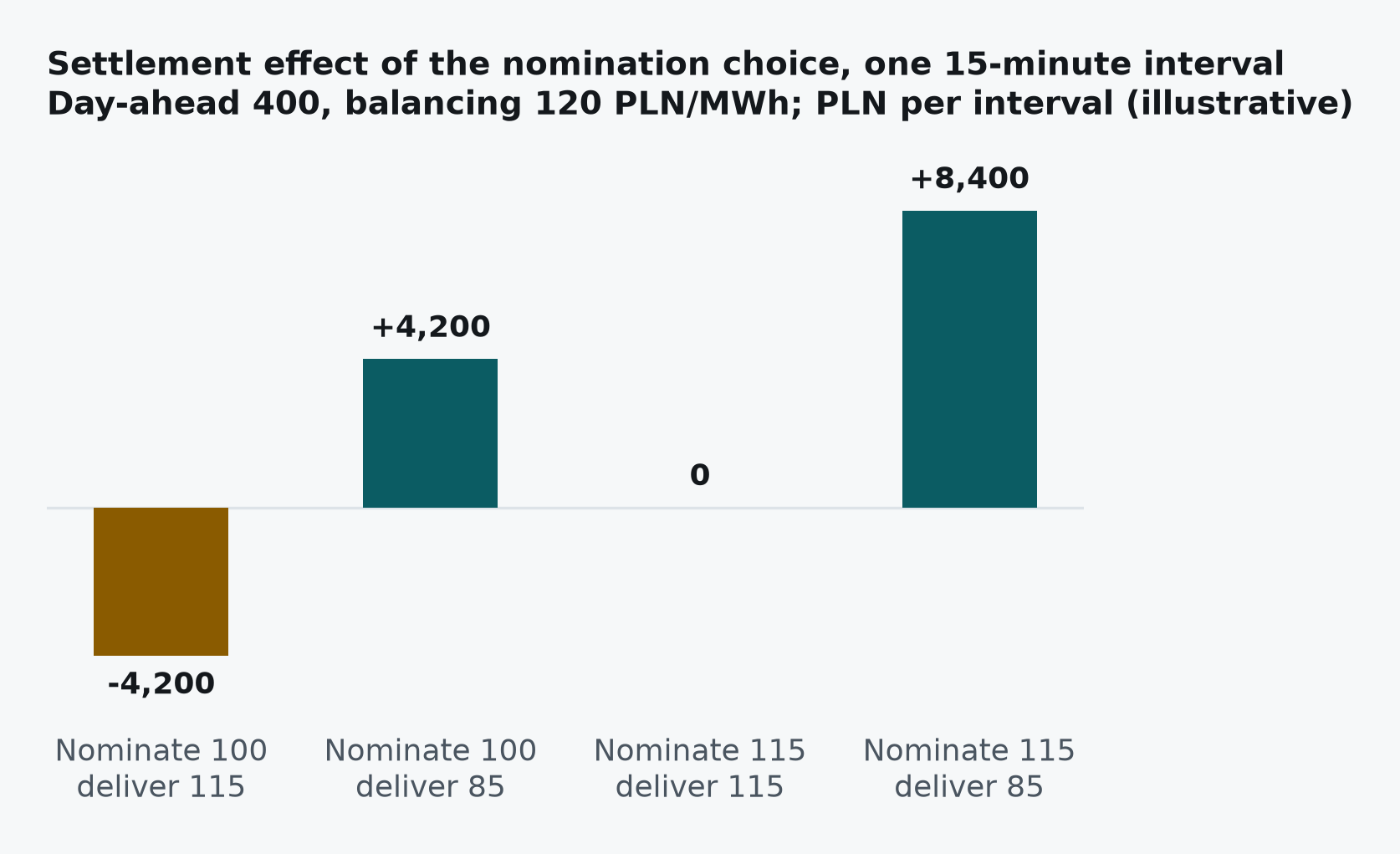
Take one wind portfolio, one 15-minute interval, a day-ahead price of 400 PLN/MWh and a balancing price of 120 PLN/MWh, with a production forecast that is genuinely uncertain between 80 and 120 MWh.

Nomination	Delivered	Error	Settlement effect
100 MWh	115 MWh	+15	15 MWh surplus settled at 120 instead of 400: cost 4,200 PLN
100 MWh	85 MWh	−15	15 MWh shortfall bought back at 120 against 400 received: gain 4,200 PLN
115 MWh	115 MWh	0	no imbalance
115 MWh	85 MWh	−30	30 MWh bought back at 120 against 400: gain 8,400 PLN

With the spread pointing this way, the rows that nominated near the top of the plausible range do at least as well as the central nomination, and the under-forecast row is the only one that loses. Put the balancing price at 700 PLN/MWh instead and every conclusion inverts: the high nomination becomes the costly one and the cautious one becomes safe. The forecast error was the same throughout. The spread decided the result.

What nomination strategy should weight

The choice of which point in the forecast’s uncertainty range to nominate is therefore a real decision with a financial answer, and the answer depends on the expected spread for that interval. When day-ahead is running well above the expected balancing price, nominating towards the upper part of the plausible range costs little if production disappoints and avoids the expensive surplus if it does not. When the expected spread points the other way, the cautious end of the range is the safe one.

Nothing in this involves producing anything other than what the weather delivers, or deviating from a nomination once made. It is a choice about where in the forecast distribution to place the nomination, taken before gate closure, in full view of the settlement rules. Stated as a general finding from simulated scenarios: a nomination rule that weights the current day-ahead-versus-balancing spread consistently outperforms one that only minimizes expected forecast error, by a margin that matters at portfolio scale.

On the Polish market this is the largest controllable component of the gap between capture price and realized value per MWh. Capture price is what day-ahead paid; realized value is what remained after the balancing market priced the forecast error, and that price is shaped far more by the spread than by the error.

Practical implications

Report realized value per MWh alongside forecast accuracy, and when the two move in opposite directions, believe the money.

Decompose imbalance cost by the sign of the error and by the sign of the spread in each interval. The decomposition usually shows that a small number of wide-spread intervals account for most of the cost.

Give the nomination process a view of the expected spread, so that the point in the forecast range it nominates is a decision and no longer a default.

Related reading

• What Intraday Liquidity Is Worth to a Renewable Portfolio — the other lever against the same imbalance settlement mechanism
• What Realized Value per MWh Actually Measures — the metric this spread ultimately moves

When you last reviewed your portfolio’s imbalance cost, was it broken down by the direction of the error and the sign of the spread, or only by the size of the error?